gVenn: Proportional Venn diagrams for genomic regions and gene set overlaps
Christophe Tav
May 2026
Source:vignettes/gVenn.Rmd
gVenn.Rmd
Introduction
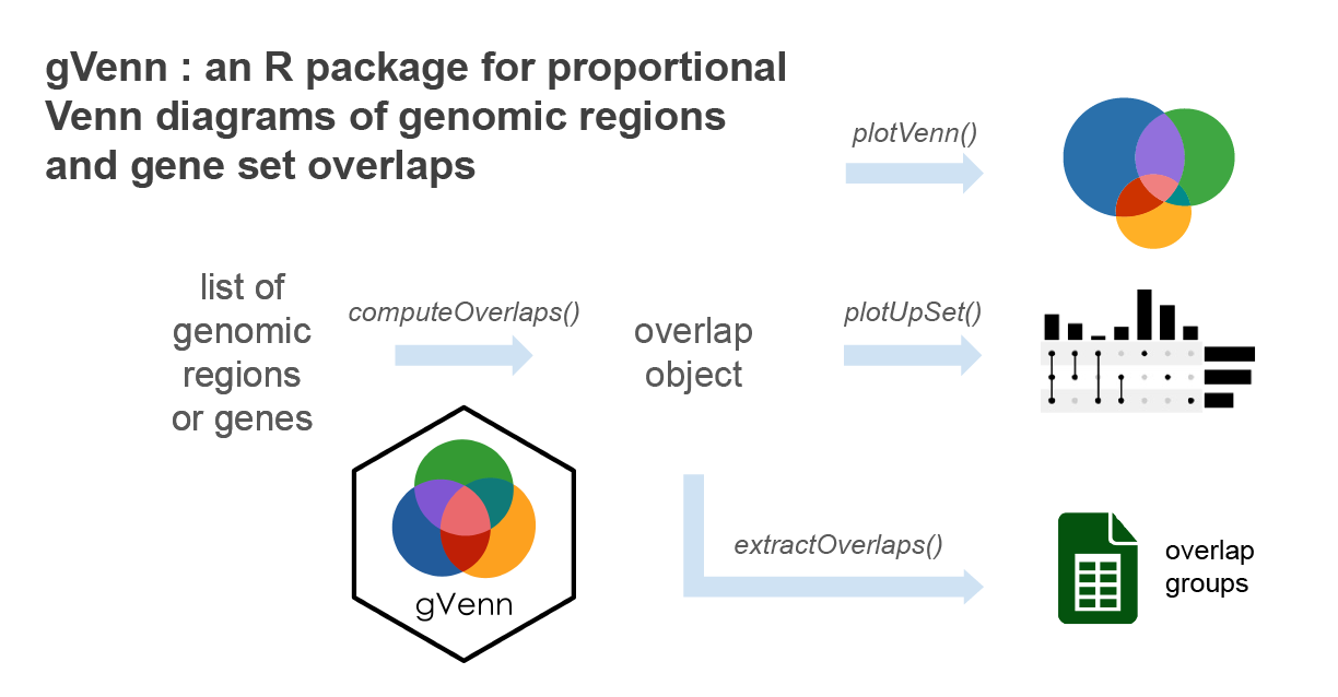
gVenn stands for gene/genomic
Venn.
It provides tools to compute overlaps between genomic regions or sets of
genes and visualize them as Venn diagrams with areas
proportional to the number of overlapping elements. In addition, the
package can generate UpSet plots for cases with many
sets, offering a clear alternative to complex Venn diagrams.
With seamless support for GRanges and
GRangesList objects, gVenn integrates
naturally into Bioconductor workflows such as ChIP-seq, ATAC-seq, or
other interval-based analyses.
Overlap groups can be easily extracted for further analysis, such as motif enrichment, transcription factor binding enrichment, or gene annotation. gVenn package produces clean, publication-ready figures.
Installation
The gVenn package is available through Bioconductor and GitHub.
You can install it from Bioconductor using:
if (!require("BiocManager", quietly = TRUE))
    install.packages("BiocManager")
BiocManager::install("gVenn")
To install the development version from GitHub, use:
# install.packages("pak")  # if not already installed
pak::pak("ckntav/gVenn")

# or, alternatively:
# install.packages("devtools")  # if not already installed
devtools::install_github("ckntav/gVenn")
Example workflow
This section demonstrates a typical workflow with gVenn, from computing overlaps to generating clean, publication-ready figures. The examples show how to work with genomic interval data.
We start by loading the package:
1. Load example ChIP-seq peak sets (genomic)
We use the dataset a549_chipseq_peaks,
which contains example consensus peak subsets for MED1,
BRD4, and GR after dexamethasone
treatment in A549 cells. To keep the dataset small and suitable for
examples and tests, each set has been restricted to peaks located on
chromosome 7.
These data originate from Tav et al. (2023) (doi:10.3389/fgene.2023.1237092).
# Load the example A549 ChIP-seq peaks (subset on chr7 for demo)
data(a549_chipseq_peaks)
2. Compute overlaps between genomic regions
We compute overlaps between the ChIP-seq peak sets using
computeOverlaps():
genomic_overlaps <- computeOverlaps(a549_chipseq_peaks)The result is a structured GenomicOverlapResult object
that contains:
- A GRanges object, where each region includes metadata describing its overlap pattern across the input sets.
- An associated logical matrix (or data frame) indicating which reduced regions overlap with which input sets.
3. Visualization
Venn diagram
plotVenn() draws proportional Venn diagrams from the
overlap object.
plotVenn(genomic_overlaps)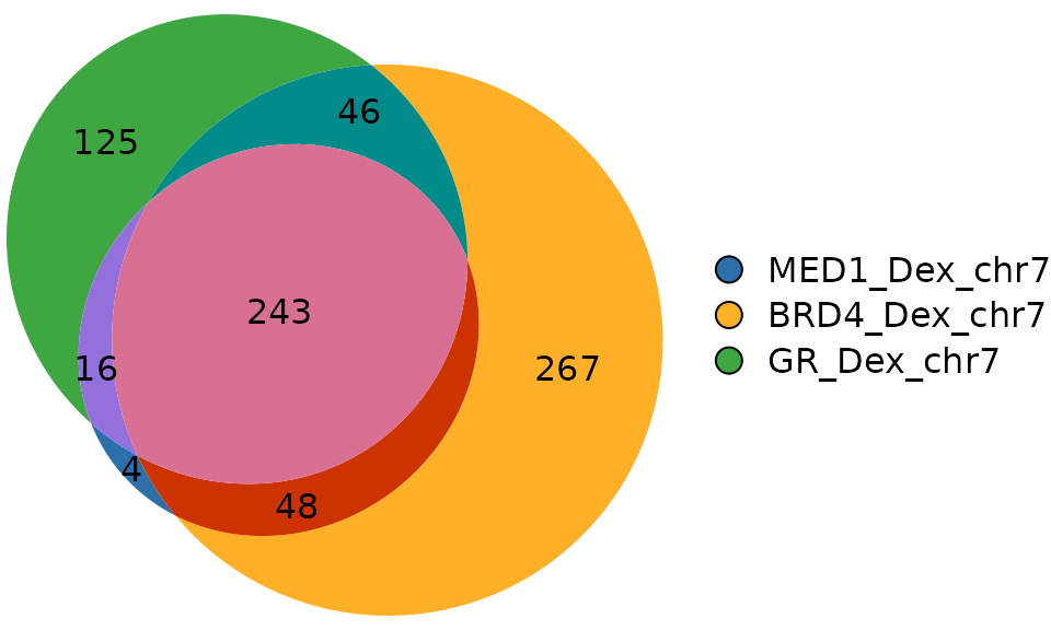
UpSet plot
For more than three sets, a Venn diagram with
areas exactly proportional to all intersections is
generally not mathematically attainable. Solvers (like
those used by eulerr) provide best-effort
approximations, but the layout can become hard to read. In
these cases, an UpSet plot is the recommended
visualization because it scales cleanly to many sets and preserves
intersection sizes precisely on bar axes.
We therefore suggest using plotUpSet() when you have
> 3 sets (or any time the Venn becomes visually
crowded).
plotUpSet(genomic_overlaps)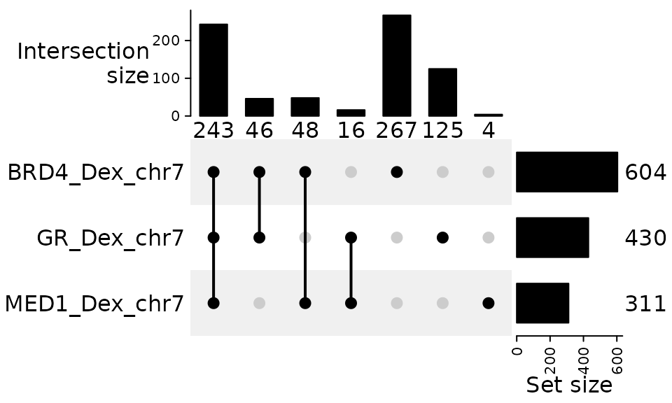
You can customize the colors of the combination matrix dots and
connecting lines using the comb_col parameter. This
parameter accepts a single color or a vector of colors:
plotUpSet(genomic_overlaps, comb_col = c( "#D87093", "#CD3301", "#9370DB", "#008B8B", "#2B70AB", "#FFB027", "#3EA742"))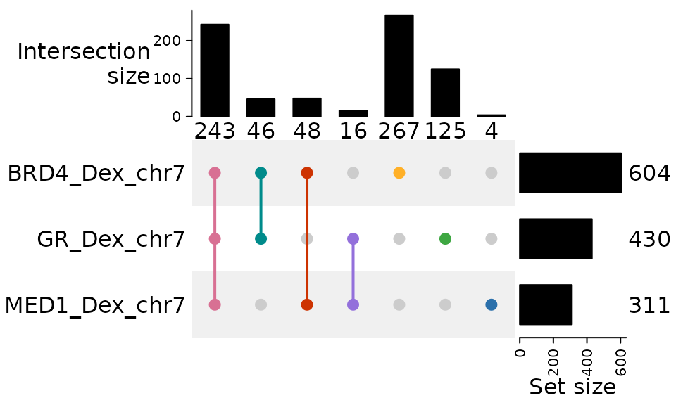
Export visualization
You can export any visualization using saveViz():
venn <- plotVenn(genomic_overlaps)
saveViz(venn,
        output_dir = ".",
        output_file = "figure_gVenn",
        format = "pdf")
By default, files are written to the current directory (“.”). If you enabled the date option (today), the current date will be prepended to the filename.
You can also export to PNG or SVG:
# png
saveViz(venn,
        output_dir = ".",
        output_file = "figure_gVenn",
        format = "png")

# pdf
saveViz(venn,
        output_dir = ".",
        output_file = "figure_gVenn",
        format = "svg")
By default, the background is white. For presentations or
publications with colored backgrounds, figures can be exported with a
transparent background using bg = "transparent":
4. Extract elements per overlap group
groups <- extractOverlaps(genomic_overlaps)
# Display the number of genomic regions per overlap group
sapply(groups, length)
#> group_010 group_001 group_100 group_110 group_011 group_101 group_111
#>       267       125         4        48        46        16       243
In this example:
- 243 peaks are shared across all three factors (MED1, BRD4, and GR)
- 267 peaks are unique to BRD4
- 48 peaks are shared between MED1 and BRD4 only
Overlap group naming
When overlaps are computed, each group of elements or genomic regions is labeled with a binary code that indicates which sets the element belongs to.
- Each digit in the code corresponds to one input set (e.g., A, B, C).
- A 1 means the element is present in that set, while 0 means absent.
- The group names in the output are prefixed with “group_” for clarity.
| Group name | Meaning |
|---|---|
group_100 |
Elements only in A |
group_010 |
Elements only in B |
group_001 |
Elements only in C |
group_110 |
Elements in A ∩ B (not C) |
group_101 |
Elements in A ∩ C (not B) |
group_011 |
Elements in B ∩ C (not A) |
group_111 |
Elements in A ∩ B ∩ C |
Extract one particular group
Each overlap group can be accessed directly by name for downstream analyses, including motif enrichment, transcription factor (TF) enrichment, annotation of peaks to nearby genes, functional enrichment or visualization.
For example, to extract all elements that are present in A ∩ B ∩ C:
# Extract elements in group_111 (present in all three sets: MED1, BRD4, and GR)
peaks_in_all_sets <- groups[["group_111"]]

# Display the elements
peaks_in_all_sets
#> GRanges object with 243 ranges and 1 metadata column:
#>         seqnames              ranges strand | intersect_category
#>            <Rle>           <IRanges>  <Rle> |        <character>
#>     [1]     chr7     1156721-1157555      * |                111
#>     [2]     chr7     1520256-1521263      * |                111
#>     [3]     chr7     2309811-2310529      * |                111
#>     [4]     chr7     3027924-3028466      * |                111
#>     [5]     chr7     3436651-3437214      * |                111
#>     ...      ...                 ...    ... .                ...
#>   [239]     chr7 158431413-158433728      * |                111
#>   [240]     chr7 158818200-158819318      * |                111
#>   [241]     chr7 158821076-158821876      * |                111
#>   [242]     chr7 158863108-158864616      * |                111
#>   [243]     chr7 159015311-159016245      * |                111
#>   -------
#>   seqinfo: 24 sequences from an unspecified genome; no seqlengths
Export overlap groups
Each overlap group (e.g., group_100,
group_110, group_111) can be exported for
downstream analysis. The gVenn package provides two export functions
depending on your data type and downstream needs:
For all overlap types (genomic or gene sets):
The function exportOverlaps() writes each group to an
Excel file with one sheet per overlap group, making it easy to review
and reuse the results outside of R.
# export overlaps to Excel file
exportOverlaps(groups,
               output_dir = ".",
               output_file = "overlap_groups")
For genomic overlaps only:
When working with genomic regions (GRanges objects), you can export
overlap groups as BED files using exportOverlapsToBed().
This creates one BED file per overlap group, which is ideal for
visualization in genome browsers (IGV, UCSC Genome Browser) or for
downstream analyses requiring BED format input.
# Export genomic overlaps to BED files
exportOverlapsToBed(groups,
                    output_dir = ".",
                    output_prefix = "overlaps")

# This will create separate BED files such as:
# - overlaps_group_100.bed
# - overlaps_group_110.bed
# - overlaps_group_111.bed
# etc.
Customization examples
This section shows common ways to customize the Venn diagram produced
by plotVenn(). All examples use the built-in
gene_list dataset.
# load the example gene_list
data(gene_list)

# compute overlaps between gene sets
res_sets <- computeOverlaps(gene_list)

# basic default venn plot (uses package defaults)
plotVenn(res_sets)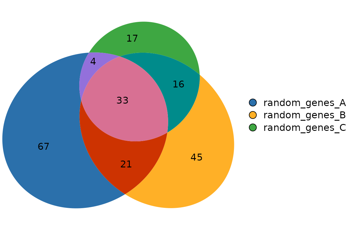
Custom fills with transparency
plotVenn(res_sets,
         fills = list(fill = c("#FF6B6B", "#4ECDC4", "#45B7D1"), alpha = 0.5),
         legend = "right",
         main = list(label = "Custom fills (transparent)", fontsize = 14))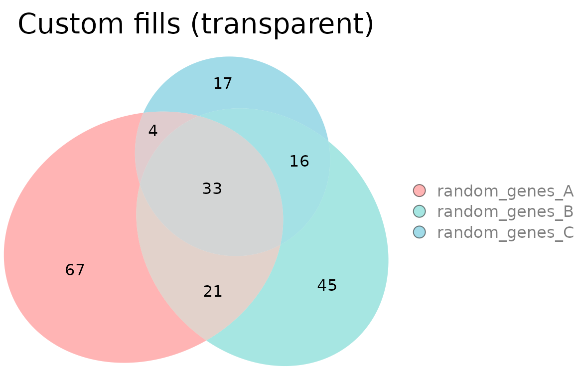
Colored edges, no fills (colored borders only)
plotVenn(res_sets,
         fills = "transparent",
         edges = list(col = c("red", "blue", "darkgreen"), lwd = 2),
main = list(label = "Colored borders only"))![]()
Custom labels and counts + percentages
plotVenn(res_sets,
         labels = list(col = "black", fontsize = 12, font = 2),
         quantities = list(type = c("counts","percent"),
                           col = "black", fontsize = 10),
         main = list(label = "Counts + Percentages", fontsize = 14))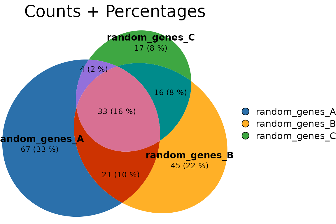
Legend at the bottom with custom text
plotVenn(res_sets,
         legend = list(side = "bottom",
                       labels = c("Treatment A","Treatment B","Control"),
                       fontsize = 10),
         main = list(label = "Custom legend"))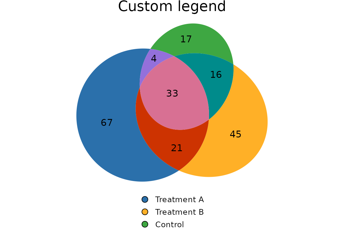
Combining multiple custom options
plotVenn(res_sets,
         fills = list(fill = c("#2B70AB", "#FFB027", "#3EA742"), alpha = 0.6),
         edges = list(col = "gray30", lwd = 1.5),
         labels = list(col = "black", fontsize = 7, font = 2),
         quantities = list(type = "counts", col = "black", fontsize = 10),
         main = list(label = "multiple custom options Venn", fontsize = 16, font = 2),
         legend = FALSE)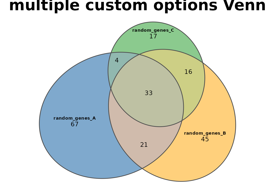
Session info
This vignette was built with the following R session:
sessionInfo()
#> R version 4.6.0 (2026-04-24)
#> Platform: x86_64-pc-linux-gnu
#> Running under: Ubuntu 24.04.4 LTS
#>
#> Matrix products: default
#> BLAS:   /usr/lib/x86_64-linux-gnu/openblas-pthread/libblas.so.3
#> LAPACK: /usr/lib/x86_64-linux-gnu/openblas-pthread/libopenblasp-r0.3.26.so;  LAPACK version 3.12.0
#>
#> locale:
#>  [1] LC_CTYPE=C.UTF-8       LC_NUMERIC=C           LC_TIME=C.UTF-8
#>  [4] LC_COLLATE=C.UTF-8     LC_MONETARY=C.UTF-8    LC_MESSAGES=C.UTF-8
#>  [7] LC_PAPER=C.UTF-8       LC_NAME=C              LC_ADDRESS=C
#> [10] LC_TELEPHONE=C         LC_MEASUREMENT=C.UTF-8 LC_IDENTIFICATION=C
#>
#> time zone: UTC
#> tzcode source: system (glibc)
#>
#> attached base packages:
#> [1] stats4    stats     graphics  grDevices utils     datasets  methods
#> [8] base
#>
#> other attached packages:
#> [1] gVenn_1.3.2          GenomicRanges_1.64.0 Seqinfo_1.2.0
#> [4] IRanges_2.46.0       S4Vectors_0.50.1     BiocGenerics_0.58.1
#> [7] generics_0.1.4
#>
#> loaded via a namespace (and not attached):
#>  [1] eulerr_7.1.0          sass_0.4.10           shape_1.4.6.1
#>  [4] polylabelr_1.0.0      stringi_1.8.7         magrittr_2.0.5
#>  [7] digest_0.6.39         evaluate_1.0.5        grid_4.6.0
#> [10] timechange_0.4.0      RColorBrewer_1.1-3    iterators_1.0.14
#> [13] circlize_0.4.18       fastmap_1.2.0         foreach_1.5.2
#> [16] doParallel_1.0.17     jsonlite_2.0.0        GlobalOptions_0.1.4
#> [19] ComplexHeatmap_2.28.0 codetools_0.2-20      textshaping_1.0.5
#> [22] jquerylib_0.1.4       cli_3.6.6             rlang_1.2.0
#> [25] crayon_1.5.3          polyclip_1.10-7       cachem_1.1.0
#> [28] yaml_2.3.12           tools_4.6.0           parallel_4.6.0
#> [31] colorspace_2.1-2      GetoptLong_1.1.1      vctrs_0.7.3
#> [34] R6_2.6.1              png_0.1-9             matrixStats_1.5.0
#> [37] lifecycle_1.0.5       lubridate_1.9.5       stringr_1.6.0
#> [40] fs_2.1.0              clue_0.3-68           cluster_2.1.8.2
#> [43] ragg_1.5.2            desc_1.4.3            pkgdown_2.2.0
#> [46] bslib_0.11.0          glue_1.8.1            Rcpp_1.1.1-1.1
#> [49] systemfonts_1.3.2     xfun_0.57             knitr_1.51
#> [52] rjson_0.2.23          htmltools_0.5.9       rmarkdown_2.31
#> [55] compiler_4.6.0
References
Example A549 ChIP-seq dataset
- Tav, C., Fournier, É., Fournier, M., Khadangi, F., Baguette, A., Côté, M.C., Silveira, M.A.D., Bérubé-Simard, F.-A., Bourque, G., Droit, A., & Bilodeau, S. (2023). Glucocorticoid stimulation induces regionalized gene responses within topologically associating domains. Frontiers in Genetics, 14, 1237092. doi:10.3389/fgene.2023.1237092
Supporting packages
eulerr : Larsson, J. (2023). eulerr: Area-Proportional Euler and Venn Diagrams with Ellipses. CRAN package page
ComplexHeatmap : Gu, Z., Eils, R., & Schlesner, M. (2016). Complex heatmaps reveal patterns and correlations in multidimensional genomic data. Bioinformatics, 32(18), 2847–2849. doi:10.1093/bioinformatics/btw313